Statistics: error bars for time averages#
This page explains what polyphys.analyze.stats estimates, how to
read its blocking table, how to choose the plateau, and when the naive
standard error is still the right one.
Notation#
- \(x_t\)
The value of one observable at frame \(t = 1, \dots, n\).
- \(n\)
The number of frames,
n_frames.- \(\sigma^2\)
The variance of \(x_t\) over the frames, with
ddof=1; \(\sigma\) is its standard deviation.- \(k\)
The blocking level, \(k = 0, 1, 2, \dots\).
- \(B\)
The block size in frames at level \(k\), \(B = 2^k\).
- \(m\)
The number of blocks at that level, \(\lfloor n / B \rfloor\).
- \(\mathrm{SE}(B)\)
The standard error of the mean estimated from the \(m\) block means; \(\mathrm{SE}(1) = \sigma / \sqrt{n}\) is the naive estimate.
- \(s(B)\)
The statistical inefficiency estimated at block size \(B\): the variance of the block means times \(B\), divided by \(\sigma^2\). When \(n\) is a power of two, \(s(B) = (\mathrm{SE}(B) / \mathrm{SE}(1))^2\).
- \(s\)
The statistical inefficiency, the plateau of \(s(B)\) at block sizes beyond the correlation time: the number of frames that make one independent sample.
- \(\rho(t)\)
The normalized autocorrelation function of \(x_t\) at a lag of \(t\) frames, with \(\rho(0) = 1\); for a stationary series \(s = \sum_{t=-\infty}^{\infty} \rho(t)\).
- \(\tau_\mathrm{int}\)
The integrated autocorrelation time in Wolff’s (2004) convention, \(\tau_\mathrm{int} = s / 2\), in frames.
- \(\phi\), \(\epsilon_t\)
The coefficient and the independent unit-variance noise of an AR(1) series, \(x_t = \phi x_{t-1} + \epsilon_t\) with \(|\phi| < 1\), used in the figures; its inefficiency is \(s = (1 + \phi) / (1 - \phi)\).
- \(R\)
The number of independent replicates of one state point.
The sections below also define each symbol where it first appears.
Two kinds of average#
A PolyPhys measurement is averaged twice: over the frames of one run (a
whole), and over the independent runs of one state point (an ensemble).
The two averages need different error bars.
Average |
Samples |
Independent? |
Error estimator |
|---|---|---|---|
Time average |
the frames of one trajectory |
no |
block averaging, |
Ensemble average |
the time averages of replicate runs |
yes |
the naive standard error, |
Consecutive frames of a polymer trajectory are correlated over at least the
chain’s longest relaxation time, and longer under confinement or crowding. For
a series of \(n\) frames whose values have standard deviation \(\sigma\), the
textbook standard error, \(\sigma / \sqrt{n}\), treats every frame as a new
observation, so it understates the error of a time average by
\(\sqrt{s}\), where \(s\) is the statistical inefficiency, the number of frames
that make one independent sample. Replicates started from independent seeds
are independent, so across them the naive estimator is correct;
ens_avg_from_df() keeps it.
The blocking method#
Flyvbjerg and Petersen (1989) replace the series by the means of consecutive
pairs of frames, then pairs of pairs, and so on, and recompute the standard
error of the mean at each level. At level \(k = 0, 1, 2, \dots\) the block size
is \(B = 2^k\) frames and there are \(m = \lfloor n / B \rfloor\) blocks; the
standard error estimated from the \(m\) block means is written
\(\mathrm{SE}(B)\), so \(\mathrm{SE}(1) = \sigma / \sqrt{n}\) is the naive value.
The estimated inefficiency \(s(B)\) is \(B\) times the variance of the block
means divided by \(\sigma^2\), which is \((\mathrm{SE}(B) / \mathrm{SE}(1))^2\)
when \(n\) is a power of two. Blocks shorter than the correlation time, the lag
over which the series’ autocorrelation decays, give too small an estimate;
once the blocks are longer than it, the block means are effectively
independent and the estimate stops growing. The plateau of \(\mathrm{SE}(B)\) is
the error bar of the time average, and the plateau of \(s(B)\) is \(s\). block_average()
returns the whole table as a BlockingResult:
import numpy as np
from polyphys.analyze.stats import block_average

rg = np.load("rg_timeseries.npy")      # shape (n_frames,), after equilibration
table = block_average(rg)
for size, count, se, err, s in zip(
    table.block_size, table.n_blocks, table.sem, table.sem_err,
    table.statistical_inefficiency,
):
    print(f"{size:6d} {count:7d} {se:9.4f} +- {err:7.4f}   s = {s:6.2f}")
Reading the table:
block_sizedoubles at each level;n_blockshalves, dropping an unpaired trailing block when the count is odd.semis the standard error of the mean using the block means as the sample. Level 0 is the naive estimate. Where it stops rising, withinsem_err, is the plateau.statistical_inefficiencyisblock_size * var / var[0]: it rises from 1 and plateaus at \(s\).n_frames / sis the effective number of independent frames.
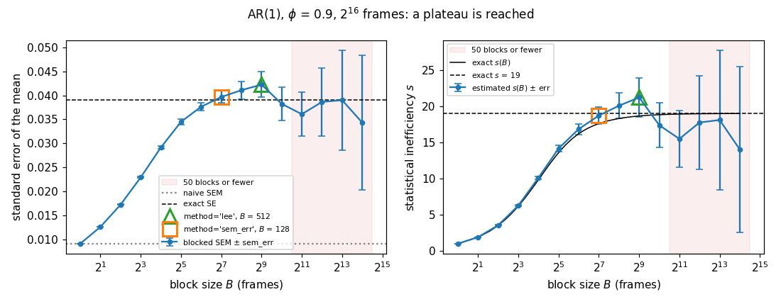
for an AR(1) series with phi 0.9; both rise and level off at the exact values, with error bars growing at large block sizes. :width: 100%#
A run long enough for a plateau: an AR(1) series, \(x_t = \phi x_{t-1} +
\epsilon_t\) with coefficient \(\phi = 0.9\) and independent unit-variance noise
\(\epsilon_t\), of \(2^{16}\) frames. Its exact inefficiency is
\(s = (1 + \phi) / (1 - \phi) = 19\). Left, the standard error rises from the naive
value (dotted) to the exact one (dashed) and levels off from \(B \approx 128\).
Right, the estimated \(s(B)\) follows the exact curve. method='sem_err'
(square) stops at the start of the plateau, method='lee' (triangle) two
levels later; both agree with the exact value within their error bars. In the
shaded region 50 blocks or fewer remain and the points scatter.
At the deepest levels only a few blocks remain and
sem_erris large; those rows are noise, not plateau.min_blocks(default 4) sets where the table stops.
The input may have any trailing shape: (n_frames, n_bins) for a per-frame
histogram gives one column of the table per bin, and the selectors below
return one level per bin.
Choosing the plateau#
Which level to report is an estimator choice, so the module offers three ways and never picks one silently.
- (a) Read the table
Flyvbjerg and Petersen’s own practice. Look at
semagainstblock_sizeand take the plateau by eye, withsem_erras the error bar on each entry.- (b)
method="lee" The rule of Lee et al. (2011), Eq. (14), as the
pyblockpackage implements it. Scanning from the largest block downward, a level qualifies when its block size satisfies \(B^3 > 2 n (\mathrm{SE}(B) / \mathrm{SE}(1))^4\), and the selected level is the smallest block of the qualifying run that reaches the top. The rule balances the systematic underestimate at small blocks against the growing statistical error at large ones. Wolff (2004), Eq. (47), derives the same balance with a constant four times smaller in \(B^3\), because his correlation time is the integrated autocorrelation time \(\tau_\mathrm{int} = s / 2\) where Lee et al. use \(s\); neither constant is exact.- (c)
method="sem_err" The first level whose
semlies within onesem_errof each of the next two levels, that is, where the table first flattens. A convenience heuristic without a published source; it tends to pick the start of the plateau and so to err on the low side.
from polyphys.analyze.stats import sem_blocked, statistical_inefficiency

error_bar = sem_blocked(rg, method="lee")
s = statistical_inefficiency(rg, method="lee")
When no level qualifies, the selectors return -1 and the wrappers NaN,
with a RuntimeWarning. That is the honest answer for a run that is too
short for its correlation time, or that drifts or switches between metastable
states too rarely to sample them: the error bar of such a run cannot be
estimated from the run as it stands. More effective samples are what help:
a longer run, which adds blocks past the correlation time, or more
independent replicates.
A run can also be too short without failing outright: the table flattens
because it runs out of blocks, not because it has reached the plateau. Lee et
al. (2011) guard against this with an acceptance criterion: their optimal
block size, \(B_\mathrm{opt} = (2 n s^2)^{1/3}\) by their Eq. (14), must be
below \(n / 50\). Since \(n / B_\mathrm{opt} > 50\) amounts to \(n / s > 500\),
the criterion asks whether the run holds more than about 500 independent
samples, a property of the run rather than of the rule. So under either
method, select_plateau() takes the block size
that method="lee" selects as \(B_\mathrm{opt}\) and raises a RuntimeWarning
when it is not below \(n / 50\), or when that rule finds no level, while
still returning the selected level. method="sem_err" alone cannot tell: it
can stop where more than 50 blocks remain on a run that fails the criterion.
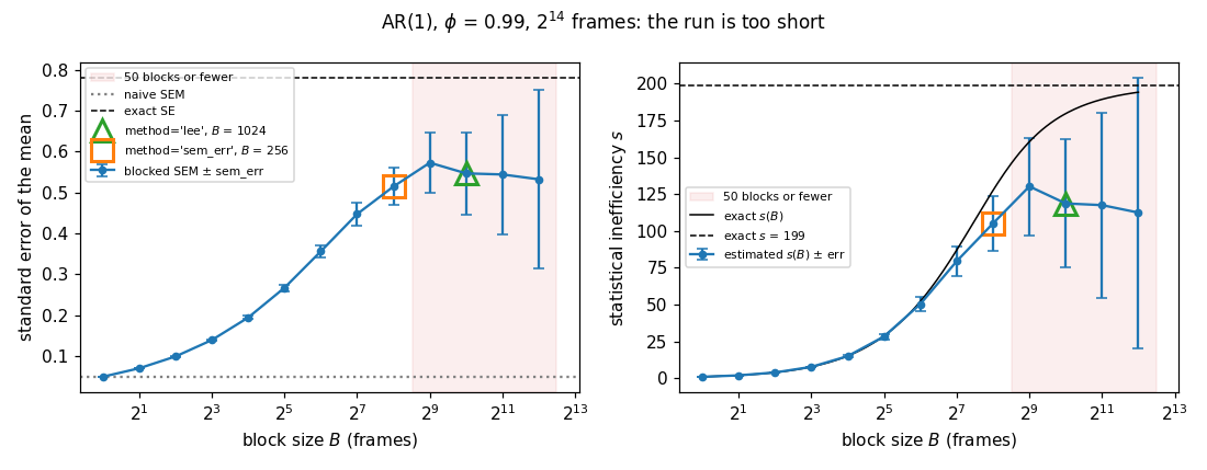
for an AR(1) series with phi 0.99 and too few frames; the estimates level off well below the exact values, inside the region with 50 blocks or fewer. :width: 100%#
A run that is too short: AR(1) with \(\phi = 0.99\) and \(2^{14}\) frames, about
82 independent samples for an exact inefficiency of 199. The table levels off
near 0.55, about 30% below the exact standard error of 0.78, because the
largest blocks still contain correlated frames. Both rules pick a level on
this false plateau, and both warn: the block size of method='lee' leaves 16
blocks, although the level method='sem_err' selects still has 64. The remedy
is a longer run or more replicates, not a different rule.
Before you call it#
Discard the equilibration transient. Blocking assumes a stationary series and cannot tell a drift from a slow mode.
Block the quantity you report. For the radius of gyration \(R_g\), the error of its time average \(\langle R_g^2 \rangle\) comes from blocking the \(R_g^2\) series; it is not the blocked error of \(R_g\) transformed.
The inefficiency is in units of saved frames. A dump stride longer than the correlation time gives \(s \approx 1\), and the table confirms that the naive error was already right.
Checking the assumption with replicates#
With \(R\) independent replicates of one state point, the scatter of their time averages is an independent measurement of the error of one time average. The ratio of the standard deviation of the \(R\) per-whole means to the typical blocked standard error of one whole should be near 1, within the \(\pm 1/\sqrt{2(R-1)}\) that \(R\) replicates allow; the naive per-whole error would predict a scatter several times too small. This check uses the maintainer’s processed data (tier C on the Testing page) and is not part of the test suite.
References#
H. Flyvbjerg and H. G. Petersen, “Error estimates on averages of correlated data”, J. Chem. Phys. 91, 461-466 (1989). https://doi.org/10.1063/1.457480
U. Wolff, “Monte Carlo errors with less errors”, Comput. Phys. Commun. 156, 143-153 (2004); erratum 176, 383 (2007). https://doi.org/10.1016/S0010-4655(03)00467-3
R. M. Lee, G. J. Conduit, N. Nemec, P. López Ríos, and N. D. Drummond, “Strategies for improving the efficiency of quantum Monte Carlo calculations”, Phys. Rev. E 83, 066706 (2011); erratum 85, 029908 (2012). https://doi.org/10.1103/PhysRevE.83.066706
M. P. Allen and D. J. Tildesley, Computer Simulation of Liquids, 2nd ed. (Oxford University Press, 2017); example code
error_calc.py.J. S. Spencer,
pyblock.